Section 1: Statistics

The important part of this section is to know the formulae and to know how to use them.  Normally, concentration will be on the x-axis (independent variable) and detector response (absorbance, area, etc.) will be on the y-axis (dependent variable).

To calculate the best-fit (least squares) line, use the following steps.  Note the following:

• "x-range" means highlight the column of your x-values in your spreadsheet (likewise for other variables)
• N = number of measurements
• "Q-Pro" = Quattro Pro (Wordperfect spreadsheet), Excel is Microsoft's spreadsheet program.  To use, click the "=" sign and type in the formula

Step	Description	Formula(s)	Spreadsheet Formula(s)
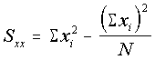
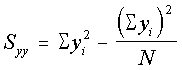
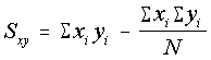
1.	Calculate the three quantities Sxx, Syy, and Sxy.		Excel: Sxx: =N*VARP(x-range)           Syy: =N*VARP(y-range) Q-pro: Sxx: =N*@VAR(x-range)            Syy: =N*@VAR(y-range) (Sxy is not required if using a spreadsheet)
2.	Using these quantities, the slope (m) of the least-squares line is	m = Sxy / Sxx	=slope(y-range, x-range)  (@slope for Q-Pro)
	The y-intercept (b) is	where the barred y and x represent the arithmetic means of y and x.	=intercept(y-range, x-range)   (@intercept for Q-Pro)
3.	The concentration of the unknown is now found by solving for x in the least-squares equation	xu = [unk] = (yu -b) / m
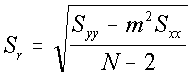
4.	To get an estimate of the error (range of values) in the regression line is given by Sr		=steyx(y-range, x-range)   (@steyx for Q-Pro)
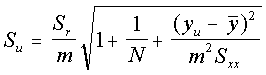
5.	An estimate of the confidence range of the unknown concentration is

• For a spiking experiment, plot data as detector response (y) vs. spiking volume added (x)
• use the following to find [unk] and its confidence range
• Note: Vu = volume of the unknown before spiking, c_s = concentration of spiking solution

3.	Find the unknown concentration cu.
5.	Find the x-intercept	x-intercept = -b / m
	Find the confidence range

Last updated, February 16, 2004
Page maintained by Craig MacKinnon